MCMC for a logistic fit from early data

Following up the Fisher information post: simulate early data from a logistic, sample the posterior with MCMC, and see how little the data say about the limiting value.

In the last post, we looked at how well early data can pin down the limiting value of a logistic curve using Fisher information. Here, we’ll use MCMC¹ to look at the distribution empirically and visualize what’s happening. The details, and all the numbers, are in the notebook.

Looking at the equation again,

\[ y(t) = \frac{L}{1 + e^{-k(t - t_0)}} = \frac{L A e^{kt}}{L + A e^{kt}}, \qquad A = L e^{-k t_0}. \]

The main variables are \(A, k, L\). If we have data that fits the exponential model well, it means that we can fit \(A, k\) well to the data.

Looking at how we define \(A = L e^{-k t_0}\), or \(\log L = \log A + k t_0\), it means that once \(A\) and \(k\) are fitted we could view \(L\) and \(t_0\) interchangeably. \(t_0\) is the inflection point, the turning point that Castro et al. (2020) found cannot be precisely forecast.

So one way we can try to see the problem of discerning between the exponential model and the logistic model from the data is to ask how well we can infer \(t_0\), given the last observation time \(T\).²

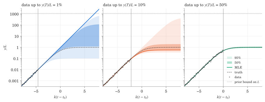
For concreteness, we take the model from the previous post with \(L = 1\), \(k = 1\), \(t_0 = 0\), 10% noise and 10 observations per \(e\)-folding time. We simulate one dataset, and cut it off at successive \(T\) as if watching the data come in.

One thing the simulation forces on us. As \(L \to \infty\) the logistic becomes the exponential, so the likelihood never goes to zero, and a flat prior on \(\log L\) can’t be normalized. So the prior has to stop somewhere, and I put it at about 1000 times the true value.

Figure 1: The maximum-likelihood fit, and the 50% and 95% posterior bands of \(y(t)\), with data up to 1%, 10% and 50% of the limit. The vertical line is the last observation.

Source: MCMC for a logistic fit from early data: the notebook

At 1% the best fit is the exponential itself, and the posterior runs up to the prior bound. At 10% it still does. By the inflection point it has closed in.

Putting \(A, k, t_0, L\) against each other,

Figure 2: Posterior of \(A\), \(k\), \(t_0\) and \(L\) at the same three cutoffs. Dashed lines are the true values, and each histogram is scaled to its own peak.

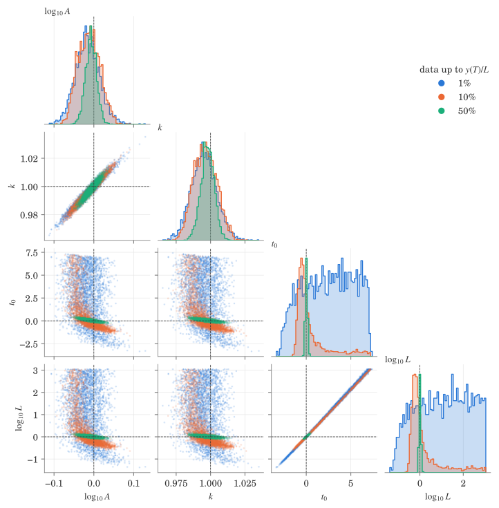
This shows we have not much information about \(t_0, L\), while \(A\) and \(k\) are pinned down even at 1%. And \(t_0\) and \(\log L\) lie on a line, as they should.

Now all seven cutoffs, as the data come in. Since there is no real prior on \(L\) here, I’d rather take the maximum-likelihood estimate as the point estimate, with a profile-likelihood interval, which needs no prior at all. The posterior is shown next to it.

Figure 3: Posterior (violins), maximum-likelihood estimate (dots) and 95% profile-likelihood interval (bars) of the limit \(L\) and of how far ahead of the last observation the turning point is, as the data come in. Arrows are intervals that do not close; the dashed lines are the truth.

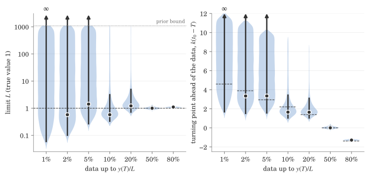
Up to 5% of the limit, the only thing the data can tell you is a lower bound, since a limit close to the data would already show as bending. At 10–20% the likelihood interval closes, but the posterior still reaches the prior bound. A likelihood that is low but flat over three decades of \(L\) still holds a lot of posterior mass, so the upper end of the credible interval there is set by the prior. By the inflection point everything agrees.

How does this compare with the equations in the last post?

Figure 4: Spread of \(\log L\) from the simulation against the Cramér–Rao bounds of the last post.

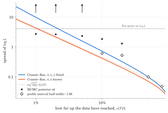
Past the inflection point the simulation agrees with the Cramér–Rao bound. Before it, the discrepancy is mainly driven by the non-Gaussianity. The bound is local, as the footnote in the last post warned, and the likelihood here is anything but Gaussian.

So before the inflection point, early data give you a lower end on \(L\), and the upper end is whatever prior you put in.

This is also why MCMC is so powerful. MCMC can be used to estimate any model we can write down, not only those we can solve analytically. Here the Fisher information could only give a local bound, and the MCMC showed the whole posterior. It has some limitations. The early part of the chain is still not representing the distribution, so it needs to be dropped carefully, and reaching the steady state that represents the actual distribution can be numerically difficult to achieve. The flat direction in \(\log L\) here is an example, which is why the notebook doesn’t use emcee’s default move. But once we iron out these issues, it is a pretty universal tool to get a statistical answer, as long as we can write down a model and compute its likelihood.

References

Castro, Mario, Saúl Ares, José A. Cuesta, and Susanna Manrubia. 2020. “The Turning Point and End of an Expanding Epidemic Cannot Be Precisely Forecast.” Proceedings of the National Academy of Sciences 117 (42): 26190–96. https://doi.org/10.1073/pnas.2007868117.

Footnotes

1. Strictly speaking, simulating the data is plain Monte Carlo. The MCMC is in the inference: it samples the posterior of the parameters given one simulated dataset.

2. I.e. we have only observed data up to time \(T\), the cutoff in the last post.